Business Analysis
Business Analysis Access/Download Help License +bizpep.com
Business Analysis will quickly build a forecast for your business (up to 10 years), determine the business value, break even point and optimum price point. It consists of 4 analysis modules Business Forecast Analysis, Business Valuation, Business Break Even Analysis and Business Pricing Analysis and runs directly in your web browser as a web page.
Give it a try it's free to review... Quick Start instructions provide a basic operational overview.
As alternatives to our browser based Business Analysis application we also have a spreadsheet based Business Valuation application providing a forecast and valuation for your business, and spreadsheet based Price Break Even Analysis to determine business breakeven and optimum pricing.
Business Forecast
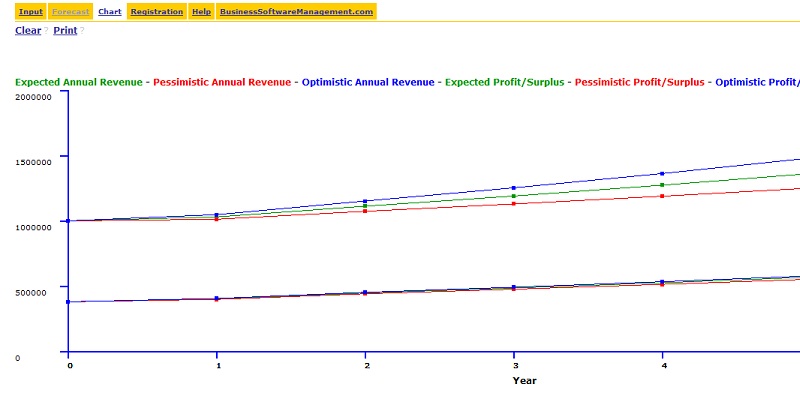
The Business Forecast module generates a forecast to assess business performance for up to a 10 year period. The forecast is built by considering future changes in the macro and micro business environment and the impact on current business performance. From this basic data future revenue and costs are determined. Sensitivity Analysis (Optimistic, Expect and Pessimistic) can be applied to the generated forecast allowing a range of scenarios to be easily tested. This forecast provides a high level strategic budget overview, assists in the identification of business opportunities and risks, and delivers a quantifiable framework for business development strategies and actions.

Developing a business forecast provides management with strategic and operational insight leading to improved business performance. It is the basis of budgeting and provides the information that allows managers to manage. Without a business forecast a business is simply responding to the day to day operating environment and has limited capacity to maximize future opportunities or minimize potential risk.
What is a Business Forecast
A Business Forecast is a prediction of a businesses future financial performance. It includes forecasts for revenue and expenses from which future profitability can be determined. It is not a detailed breakdown of revenue and expense items (as in a budget) but a higher level view of the business considering the main drivers of business revenue and expenses.
The term Sales Forecasting is often used where a forecast only encompasses the revenue component of a business forecast.
Benefits of a Business Forecast
Building a Business forecast provides insight into both the current and future performance of a business. Building a forecast should involve an assessment of the dynamic environment in which the business operates. Simply considering these issues often allows a business manager to perceive the business in a more strategic manner. This has the capacity to improve decision making and the overall strategic development of the business.
A Business Forecast can (and should be) the precursor to budget development. Developing an overall forecast and using this as a frame work for budget creation improves budget accuracy. This occurs due to the quantifiable approach applied in a valid forecast. It is not simply changing the revenue or expense by some arbitrary percentage. Instead a forecast considers changes in the factors that influence the revenue or expense and uses these to calculate the future value.
The impact of business decisions on business performance can be analyzed using a forecast. This includes decisions related directly to the business micro environment eg products and services offered and the macro environment eg changes in the target market.
Sensitivity Analysis applied to a business forecast allows a range of possible outcomes to be reviewed. Providing worst case to best case scenarios and allowing the business manager to assess, monitor and implement actions to best deal with these possibilities.
In essence a business forecast provides a high level strategic budget overview, assists in the identification of business opportunities and risks, and provides a quantifiable framework for the development of business strategies and actions.
Building a Business Forecast
Business Forecasting methods range from arbitrary year on year variations to complex data driven algorithms. The best choice depends upon the business being analyzed, the quality and quantity of data available, the purpose of the analysis, the analytical expertise of user, and time, usability, and cost constraints.
Where a business operates in a very stable environment and has demonstrated consistent incremental variations over a number of years it may be possible to successfully apply year on year variations directly to current business performance data. This can easily be undertaken using a spreadsheet.
At the other extreme where a volume of high quality data is available, and there are few cost or time constraints the use of complex modeling algorithms may be justified. However most businesses operate in dynamic environments, with limited hard data, and considerable time and cost constraints. Therefore building a usable and value adding forecast for these business requires a streamlined approach, that considers the business environment and requires minimal hard data. This is achieved by utilizing the intuitive business and market knowledge of the business manager/owner and converting this into quantifiable values that can be applied to basic current business performance data (ie revenue and broad expense categories) to build a business forecast.
You can freely review a Business Forecast using Business Analysis right now using Example Business data. Quick Start instructions provide a basic operational overview.
Business Valuation
The Business Valuation Module applies the base Forecast Analysis to generate a Business Valuation. It considers Owners Earning Power and the Required Return on Investment to develop a Business Valuation that reflects the potential to value add and considers the future business environment. This valuation provides strong support for business purchase, sale or financing negotiations. Outputs include up to a 10 year Forecast, Sensitivity Analysis, Investment Return, Net Present Value Analysis, and calculated Business Valuation (Expected, Optimistic and Pessimistic).
Determining the value of a business is required for buying, selling, establishing or financing a business. From an investment perspective a business is simply an asset the value of which is determined by its future returns (profits).
What is a Business Valuation
A Business Valuation is a calculation of the value of a business. This value is effectively the price a business could sell for or the maximum amount of capital that should be expended in setting up a business.
Benefits of a Business Valuation
A justifiable Business Valuation is the key negotiating tool when buying or selling a business. Without this there is no compelling logic behind the investment.
Using a business forecast that considers the dynamic environment in which the business operates and the potential for developing future opportunities is the basis of a verifiable business valuation. Applying Sensitivity Analysis allows a range of scenarios and corresponding valuations to be analyzed.
In essence a business valuation is the maximum amount of money that can be invested in a business while ensuring the required return on investment is achieved.
Determining a Business Valuation
Business Valuation methods include Industry Multiples (ie revenue times a multiple), past market prices, asset based valuations, and a range of return on investment approaches.
When considering the business return (profit) as an income stream from an investment (the amount invested in the business) the Return on Investment approach is most suited and widely applied. This approach considers the specific business performance. Using the Return on Investment approach requires a business forecast to determine future business returns. If this forecast applies market knowledge and allows business potential to be quantified a solid basis for valuation is provided.
You can freely review a Business Valuation using Business Analysis right now using Example Business data. Quick Start instructions provide a basic operational overview.
Breakeven Analysis
The Breakeven Analysis Module applies current performance data to determine breakeven points for Annual Revenue and Number of Sales. It applies the Annual Revenue, Total Variable, and Total Fixed values with the Breakeven Data values Average Sale Price and Number of Sales to calculate breakeven points. A Breakeven plot shows Annual Revenue and Total Expenses by Number of Sales. The Breakeven point is where Revenue and Expenses cross. Below this point the business surplus is negative (loss) and above this point the business surplus is positive (profit). The amount of surplus is the difference between the Annual Revenue and Total Expenses.
Break even analysis is a relatively simple and effective indicator of a businesses profit relationship to revenue and in turn number of sales. It can also provide insight into the impact of future sales volume changes on business profit.
What is Breakeven Analysis
Break-even Analysis applies business revenue, variable and fixed expenses to determine the point at which revenue equals expenses. This point is the break-even point. At the break-even point business profit is 0. Revenue above the break-even point results in a profit. Revenue below the break-even point results in a loss. The break-even point can also be expressed in terms of the number of sales.
Benefits of Breakeven Analysis
Knowing your breakeven point provides a quick and clear reference point for business performance. Below it you are making a loss above it a profit. A break-even plot also clearly displays the profit/loss relationship to revenue and number of sales.
Extending breakeven analysis we can gain further insight into the variable expense, fixed expense and profit relationship.
Looking at current data for the Example Business in the Business Analysis the Fixed Expense per unit is 17% of Revenue with the Number of Sales being 10 000 and an Average Sale Price of 100.
At the break-even point Fixed Expenses are 55% of Revenue with the Number of Sales being 3 090 and an Average Sale Price of 100.
This clearly demonstrates the reduction in per unit Fixed Expenses as the Number of Sales increases. The reduction in per unit Fixed Expenses with each additional sale results in a decreasing marginal cost for each sale made. Basically considering Fixed Expenses the next sale always provides more profit than the current sale due to the reduced Fixed Expense per unit.
However in most business operating environments each additional sale becomes a little harder (ie the easiest sales are made fist). So to complete the next sale it may require increased marketing effort or a reduced price. But as Fixed Expenses per unit decrease for each additional sale we actually have the amount of this expense reduction to either contribute to increased marketing or compensate for a price reduction without undermining our profit margin.
Performing Break-even Analysis
To calculate a businesses break-even point costs are identified as either Variable or Fixed expenses.
Variable Expenses
Variable expenses change with the volume of product or service provided. These costs include materials, production, distribution, and transaction costs. Variable expenses are incurred each time a product or service is produced or delivered. If the number of sales (product/service delivery) is 0 Variable expenses are 0.
Fixed Expenses
Fixed expenses remain constant (up to a point) while the number of sales vary. This includes administration, location, and finance costs. Fixed expenses are incurred even if the number of sales is 0.
Break-even Formula
Break-even Revenue can be calculated as:
Break-even Revenue = Total Fixed / ( 1 - (( Total Variable / Number of Sales ) / Average Sale Price ))
this is equivalent to
Break-even Revenue = Total Fixed / ( 1 - ( Variable Expense per Sale / Average Sale Price ))
Revenue less than break-even revenue results in a loss. Revenue greater than break-even revenue results in a profit.
The Break-even Number of Sales can be calculated as:
Break-even Number of Sales = Break-even Revenue / Average Sale Price
Less than the break-even number of sales results in a loss. Greater than break-even number of sales results in a profit.
You can freely review Break-even Analysis at Business Analysis right now using Example Business data. Quick Start instructions provide a basic operational overview.
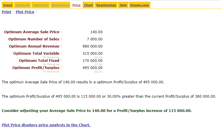
Price Analysis
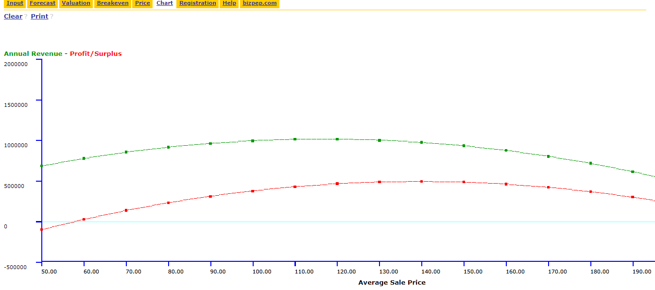
The Price Analysis Module determines the impact of a price change on your business. It applies current Annual Revenue, Total Variable, and Total Fixed values with the Price Data values Sale Price Change % and Number of Sales Change % to project business surplus over a range of prices. Price Analysis projects outcomes for pricing from 50% to 200% of the current price and calculates the optimum price. The optimum price provides the highest surplus (profit). It can be utilized to test the impact of pricing changes on revenue and surplus and identify the Optimum Pricing to maximize business surplus. A Price plot shows Annual Revenue and Profit/Surplus by Average Sale Price. The optimum Average Sale Price is where Profit/Surplus is highest. By stepping through price ranges of 50% to 200% of the current Average Sale Price, calculating the corresponding Profit/Surplus and identifying the point of maximum Profit/Surplus the optimum Average Sale Price is determined.
What is Price Analysis
Price Analysis combines the business revenue, variable and fixed expense relationship of a business with price and number of sales changes to determine the point at which the greatest profit/surplus is achieved. This is the Optimum price.
Benefits of Price Analysis
The impact of price changes and sales volume is not intuitive. Due to variable and fixed expense ratios business profit is not directly proportional to business revenue. Price analysis provides a quick and easy approach to exploring a range of price and number of sales relationships to determine the impact of price changes on business profit. A Price plot clearly displays the profit/loss relationship for prices from 50% to 200% of the current price.
Performing Price Analysis
Price Analysis is performed by using Step Values of 0.5 to 2.0 (ie 50% to 200%) of the current Average Sale Price to step through price ranges, calculating the corresponding Profit/Surplus based on the Price change data and identifying the price providing the maximum Profit/Surplus.
You can freely review Price Analysis using Business Analysis right now using Example Business data. Quick Start instructions provide a basic operational overview.
Business Analysis Access/Download Help License +bizpep.com
Access/Download Business Analysis
Business Analysis runs in your web browser as a web page and can be run directly from our server at Business Analysis with no download or installation.
![]() Business Analysis - Online web based hosted application.
Business Analysis - Online web based hosted application.
or you can download the Compressed Zip file and save to your local system
![]()
![]() Download Business Analysis - Compressed Zip file ba.zip
Download Business Analysis - Compressed Zip file ba.zip
If you download the Compressed Zip file unzip/uncompress the downloaded file and save the content .html software file. Open the .html software file in your browser and follow the Help.
This software is free of charge for evaluation. Software runs in your browser just like a normal web page. This interface format provides the highest level of protection for your system. It does not modify or change your system settings in any way. To register and enable all functions please purchase a license.
Application suitability must be independently assessed and use indicates acceptance of any and all associated risk.
Business Analysis Access/Download Help License +bizpep.com
Help Business Analysis
Quick Start instructions provide a basic operational overview. Full instructions are included. Instructions for specific items are outlined in the Index and can also be accessed by clicking the ? after an item label when using Business Analysis.
- Open the software at Business Analysis or if you downloaded to your local system open the local .html file in your browser and follow the Help.
- Click Input from the top menu. If you have purchased a license you can input data directly into the Input Module, if not you can review the Example Business data inputs.
- A Business Forecast is built by applying Revenue, Expense and Relative Indicator inputs. The forecast can be for up to 10 years and a sensitivity analysis applied to review Optimistic, Expected and Pessimistic scenarios. Click Forecast from the top menu to display the business forecast and to from here click a line item label to plot the data set on the Chart. This can be repeated to add multiple data sets.
- This Forecast is then combined with Valuation inputs to calculate a Business Valuation. Click Valuation from the top menu to display the business valuation. Valuations are calculated for Optimistic, Expected and Pessimistic forecasts. Net Present Value (NPV) is also calculated by applying the Required Return % as the Discount Rate %.
- Break-even Analysis uses the Annual Revenue, Total Variable, Total Fixed data from the Forecast and the Break-even inputs to determine the business break-even point. Click Breakeven from the top menu to display the break-even analysis. Plot Breakeven plots the break-even data displaying Revenue and Expenses by the Number of Sales. This clearly shows the level of business profit for varying sales volumes.
- Price Analysis combines Break-even Analysis and the Price inputs to calculate the Optimum pricing for the business. At the optimum price point business profit is maximized. Plot Price displays the impact that changes in price have on business revenue and profit. This clearly identifies the price point generating the greatest profit.
- When you purchase a license you can input your own data to test different scenarios and save data sets for future use.
For detailed information please refer to the rest of this Help page. Help for specific items can be accessed from the Index or by clicking the ? after an item label in the software. If you have any questions or feedback or we can help in any way please Contact Us.
Business Analysis is compact, easy to use, and requires minimal inputs. Outputs include a multi Year Forecast, Sensitivity Analysis, Investment Return, calculated Business Valuation, Breakeven and Optimum Price analysis. Business Analysis is a compilation of our Business Forecast and Business Valuation software with additional Break-even and Price Analysis modules. It has been adapted from a number of our original Excel based business models developed by bizpep.
Business Analysis can be run as a web service on our server with no download or installation requirement. If you prefer you can Download Business Analysis, save the software file and run it directly from your computer. Software runs in your browser just like a normal web page. This interface format provides the highest level of protection for your system. It does not modify or change your system settings in any way, there is no installation.
Data is only saved locally on your computer either as a cookie or a local file. Cookies can only be accessed via the system that stored them or directly from your computer, no third party can access stored cookie data. Local files can only be accessed from your computer. This provides the highest level of security for your data.
The Business Analysis modules combine Relative Indicators for future performance with basic financial data (Revenue, Variable Costs, and Fixed Costs) to analyze a business. From these inputs a Forecast for business performance is developed. The Forecast can in-turn be applied to develop a Business Valuation. Outputs include a multi Year Forecast, Sensitivity Analysis, Investment Return, calculated Business Valuation, Break-even and Optimum Price analysis.
The performance of any business is impacted by its macro and micro environment. The macro environment encompasses variables outside the control of the business. The micro environment encompasses variables within the control of the business. By understanding the impact of these factors on future performance a business can improve its decision making to maximize opportunities and minimize risk. Using relative Indicators to quantify macro and micro variables allows their impact to be incorporated into performance analysis, provides insight into their impact and acts as a measure for the outcome of potential strategies and actions.
Relative Indicators also enable management skills and competitive advantage to be incorporated into a forecast and valuation. Managers with different skill sets will result in similar businesses performing differently. Because the value of a business depends upon the return it provides and this return is impacted by management a business can have a different value to different people. Identifying areas were management can add value by applying their unique skill sets offers the opportunity to transform a business.
Applying Break-even Analysis allows the profit impact of sales variations to be visualized and addressed. It enhances appreciation of the cost and potential of Variable and Fixed expenses in relation to sales volumes. This is extended in Price Analysis which projects outcomes for pricing from 50% to 200% of the current price and calculates the optimum price. This tests the impact of pricing changes on revenue and surplus and identifies the Optimum Price to maximize business surplus.
The menu at the top of the Business Analysis modules provides access to the main Input page, each of the Analysis areas, the Chart, the Help page (this page), the Registration page and the developer web site.
This displays the main data input for analysis. Start here and input your business data.
Analysis modules Forecast, Valuation, Break-even, Price are listed along the top menu. Registration is required to fully activate the software. Registration details are emailed when you Purchase a license. Only example inputs can be applied in non registered software.
Plots the data selected from the Analysis modules.
This page. Specific Item Help can be located using the ? link following item labels in the software.
Provides the current registration status of the software. Software is available free for evaluation using an Example Business data. To fully enable the software it must be registered. To register your software Purchase license using the secure online payment link. As soon as your transaction is processed you will receive Registration Details by return email. Then click the When you have your Registration Details Click the here button and input your Registration Details. This will register and fully enable your software. Registration details are recorded as cookies on your computer. If your cookies are blocked, cleared or removed registration details and will be lost and they will need to be re-entered. To maintain registration details please ensure cookies are enabled and are not cleared or blocked.
Link to the developer web site, for contact information and support.
Current performance inputs are based on the current full year performance of the business. Broad expense categories are provided to determine the level of expenses that vary with sales (Variable Expenses) and those that don't (Fixed Expenses). A recent business taxation return will assist in determining current inputs. If required they can be adjusted to best reflect current trading.
Input for Relative Indicators should be based on your subjective views. These are translated into quantifiable values for module operation. There is no need to provide "perfect" answers. Use industry knowledge to make informed estimates. The goal is to provide a streamline tool to indicate possible outcomes. Inputs do not have to be perfect but should reasonably reflect current business operation.
These are Module specific Controls. They appear as click-able links below the Menu.
This Control hides the Current performance inputs. It is a toggle between Compress and Expand.
This Control shows the Current performance inputs. It is a toggle between Expand and Compress.
This Control allows the decimal precision (number of decimal places) of the values to be adjusted. To adjust the decimal precision click Format. You will then be prompted to enter a new decimal precision number. Then click Format Confirm.
This Control prints the current window.You can also use the browsers Print and Print Preview functions to set print variables. To do this from your browser tool bar go File, Print or File, Print Preview.
This is an identifier for the currently displayed Analysis data. The default name is Example Business. To save data for a New Business click Save with the default Example Business selected. You will then be prompted to enter a new Business Name. Input a name for the Business and then click Save Confirm. When saved the name will appear in the drop down list and the saved data can be recalled.
This is a click-able Control, it saves your input data as a cookie on your computer. To save data for a New Business click Save with the default name Example Business selected. You will then be prompted to enter a new business name. Select an existing Business Name to Save using the existing name. You cannot Save or Delete data for the Example Business.
This is a click-able Control, it loads previously saved data from a cookie on your computer. To load business data select the required Business Name and click Load.
This is a click-able Control, it deletes a cookie on your computer containing previously saved data. To delete business data select the required Business Name and click Delete.
This is a click-able Control, it exports your input data to an xml file format that can be saved as a local file on your computer. To export business data select the required Business Name and click Export. The exported data is encoded into in an xml format and displayed in a TextArea. Select All of the TextArea contents, right click the TextArea and Copy. Open a text editor (ie notepad), Paste the copied data to a new file and Save As an xml file (*.xml). Use a descriptive file name (ie jimsbusiness.xml) so you can identify the data set saved.
This is a click-able Control, it imports your input data from a previously saved xml file format on your computer. To import business data click Import, then Browse to locate and select the required previously saved .xml file. Click Import Confirm to import the xml data. This control is only functional with registered software.
Input the Revenue generated by the business for the current year.
Current expense inputs.
This is a click-able Control. This allows you to input your Expenses directly in Monetary values (Dollars, Pounds etc). It functions as a toggle control with the Percent control. The default setting is Monetary.
This is a click-able Control. This allows you to input your Expenses as a Percentage of Annual Revenue. It functions as a toggle control with the Monetary control. The default setting is Monetary.
Variable Expenses vary with the volume of product or service you provide. Only include these costs in this section and allocate them into one of the five categories.
Input the annual variable expense for materials and supplies directly related to producing your product or providing your service.
Input the annual variable expense for labor directly related to producing your product or providing your service. This should include the annual value of any labor provided by the owner that is directly related to producing your product or providing your service. Any owner labor value should reflect the effective labor effort and can be estimated as the cost of an employee who could replace the owners efforts related to producing your product or providing your service. Labor expenses should include all associated on-costs and benefits. Do not included fixed labor expenses in this value.
Input the annual variable expense for distribution of your product or service. This may include freight costs, packaging, and vehicle running costs.
Input the annual variable expense for marketing. Include advertising, promotional publications, sponsorships, client functions, and any marketing or sales expense. Marketing is not essentially a variable expense, however it is assumed that marketing does influence the level of sales and a relationship exists between the level of marketing and the level of sales. It is on this basis that it forms a component of Variable Costs.
Input any annual variable expenses not already accounted for.
This is the sum of the variable expenses. It is expressed as a monetary value and as a percentage of Annual Revenue.
Fixed Expenses remain constant (up to a point) while the volume of sales vary. Only include these costs in this section and allocate them into one of the five categories.
Input the annual fixed location expense. Include rent, power and light, maintenance, building insurance, security, and cleaning. For a business Valuation if the business owns the property then include the current market rental/lease rate for the property ie what it would cost to lease the property for a year. Do not include purchase or finance costs.
Input the annual fixed expense for labor. This should include any labor expense not already accounted for in variable costs. This should include the annual value of any labor provided by the owner that has not already been accounted for in variable costs. Any owner labor value should reflect the effective labor effort and can be estimated as the cost of an employee who could replace the owners efforts. Labor expenses should include all associated on-costs and benefits.
Input the annual fixed administration expense. Include office phone, equipment costs, and stationary.
Input the annual fixed Interest Cost. Consider only operational finance ie working capital and overdrafts. Include only the interest component of loan repayments. Principle components reflect assets. Do not include interest related to property finance for which current market rental/lease rates have been included in Location Expenses. If you are undertaking a Business Valuation it is recommended that you do not include interest related to the business purchase. Initially the business should be valued with 100% equity. This ensures the valuation provides the required return on the Total Investment. Once you have established valuation details you can then add purchase finance interest costs to determine the impact on the business.
Input any annual fixed expenses not already accounted for.
This is the sum of the fixed expenses. It is expressed as a monetary value and as a percentage of Annual Revenue.
This is the sum of the variable and fixed expenses. It is expressed as a monetary value and as a percentage of Annual Revenue.
This is Annual Revenue less Total Expenses. Profit/Surplus reflects the before tax operating profit/loss of the business for the full years trading. It represents the day to day (short term) business performance. Asset investment including property, plant and equipment are not considered.
Annual replacement costs for business assets are calculated as the replacement value of Business Assets divided by the Life of Assets. This provides for constant reinvestment to maintain the business.
Input the replacement value of physical Business Assets. Exclude property. Consider vehicles, plant and equipment.
Input the average life of the assets. The replacement value of Business Assets will be divided by the Life of Assets to provide an indication of annual asset Depreciation Allowance.
Relative Indicators are applied to quantify factors that influence future business performance. Relative Indicators for each year are applied to reflect the percentage expected change in the unit cost or strength of the factor. Each indicator is relative to the prior year. If there is no change from the previous year the Relative Indicator is 0. A 10% increase from the previous year is reflected by a relative indicator of 10. A 10% decrease from the previous year is reflected by a relative indicator of -10. Relative indicators for costs reflect changes in the base unit of the expense such as labor costs per hour or material costs per unit.Relative Indicators are required for each factor for each of the Forecast Years. If there is no change from the previous year the Relative Indicator is 0. If there is a change input the positive or negative percentage change. Revenue and Expense inputs are used with the Relative Indicators to calculate forecast values. The default value for Relative Indicators is 0, indicating no change year on year.
This Control allows the number of Forecast Years to be adjusted. To adjust the number Forecast Years click Forecast Years. You will then be prompted to enter a new Forecast Years number. Then click Forecast Years Confirm.As the number of forecast years is increased the reliability of the forecast decreases because the further into the future we look the less certain it becomes. Generally a 3 year forecast provides a solid base for analysis. The default value for Forecast Years is 3, the maximum number is 10. When Forecast Years are increased the Relative Indicators of the last year are applied as Relative Indicators for the following years added. Adjust these as required.
Input the Relative Indicator to reflect the percentage change from the previous year for this indicator. If Market Strength will remain much the same input 0, indicating no change over the previous year. If you believe it will increase by 10% then the input would be 10. If you believe it will decrease by 10% then the input would be -10. Consider market growth, technology and regulatory impacts and customer needs. Market Strength is an indicator of the overall demand for the type of product or service you provide. This indicator has a direct relationship to forecast Annual Revenue. All things being equal as market strength increases Annual Revenue increases.
Input the Relative Indicator to reflect the percentage change from the previous year for this indicator. For an increase input a positive number, a decrease a negative number or for no change 0. Consider your position in the market, and the impact of your current actions. This is a measure of your standing relative to the competition as perceived by potential consumers. If things will remain much the same input 0, indicating no change over the previous year. If you have actions to improve the position of your business by 10% then the input would be 10. This indicator has a direct relationship to forecast Annual Revenue. All thing being equal as Business Market Position increases Annual Revenue increases. Actions contributing to the business position must be substantiated and implemented to have an impact.
Input the Relative Indicator to reflect the percentage change from the previous year for this indicator. For an increase input a positive number, a decrease a negative number or for no change 0. Consider the number of competitors, competitor strategies and potential new entrants. This indicator has an inverse relationship to forecast Annual Revenue. All things being equal as the level of competition increases Annual Revenue decreases.
Input the Relative Indicator to reflect the percentage change from the previous year for this indicator. For an increase input a positive number, a decrease a negative number or for no change 0. Consider potential unit cost changes in supplier pricing for products and services used by your business, sources of supply, your bargaining power, demand for materials, and possible alternatives. This indicator has a direct relationship to all expenses except Wages, Salaries and Interest expenses. All things being equal as the unit cost of Goods and Services increases these expenses increase. In many cases this indicator is closely related to inflation.
Input the Relative Indicator to reflect the percentage change from the previous year for this indicator. For an increase input a positive number, a decrease a negative number or for no change 0. Consider market forces and availability of skilled staff. This indicator has a direct relationship to forecast Wages and Salaries expenses. When using the Valuation Module it also has a direct relationship to forecast Owners Earning Power. All things being equal as the unit Salaries and Wages costs increase these expenses increase.
Input the Relative Indicator to reflect the percentage change from the previous year for this indicator. For an increase input a positive number, a decrease a negative number or for no change 0. This is percentage change not actual values. For a current interest rate of 5% a relative indicator of 10 in Year 1 equates to an actual interest rate of 5.5% (5% * 1.1), a relative indicator of 10 in Year 2 takes this to 6.05% (5.5 * 1.1). This indicator has a direct relationship to forecast Interest expense. All things being equal as interest rates increase this expense increases. If the business has no Interest Expense then Relative Indicator Interest Rates has no impact and can be left as 0.
Input the Relative Indicator to reflect the percentage change from the previous year for this indicator. For an increase input a positive number, a decrease a negative number or for no change 0. This should reflect changes in the relationship between your Variable Expenses and revenue. If you have actions to improve your Variable Expenses Efficiency (decrease variable expenses) by 10% over the previous year input 10. Consider changes in production, distribution and marketing processes and supplies. This indicator has an inverse relationship to all forecast Variable Expenses. All things being equal, as Variable Expenses Efficiency increases, less Supplies, Wages, Distribution and Marketing resources are required to produce the same revenue resulting in a decrease in these expenses. Actions must be substantiated and implemented to have an impact.
Input the Relative Indicator to reflect the percentage change from the previous year for this indicator. For an increase input a positive number, a decrease a negative number or for no change 0. Consider changes in administration processes, management structures and location utilization. Factors related to financing levels and requirements such as credit arrangements, debt collection and working capital are also relevant. This indicator has an inverse relationship to all forecast Fixed Expenses. All things being equal as Fixed Expenses Efficiency increases less administration, finance, management and location resources are required to produce the same revenue resulting in a decrease in these expenses. Actions must be substantiated and implemented to have an impact.
Input the Relative Indicator to reflect the percentage flow on of fixed expenses for a 100% increase in revenue. If you believe the business has surplus Fixed Expense resources (ie administration, management, location and finance utilization is less than 100%) and revenue variations will have no impact on Fixed Expenses input 0. To provide for an increase in Fixed Expenses to handle increased Revenue input a positive number. A negative number would indicate that Fixed Expenses will decrease with Revenue increases, in most cases this would not be applicable. This indicates the estimated level of Fixed Expense adjustment required to support revenue variations. Fixed Expenses are generally considered a constant expense, however large sustained revenue variations place pressure on fixed expense resources and usually result in an increase in fixed expenses. This may include larger floor area, more administration costs or higher financing. The Fixed Expense Flow-on is the percentage of increase in Fixed Expenses for a 100% increase in revenue. A Fixed Expense Flow-on of 20 reflects a 20% increase in Fixed Costs expense for every 100% increase in Annual Revenue. This indicator has a direct relationship to all forecast Fixed Expenses.
Input the percentage change in Relative Indicators utilized to generate an Optimistic and Pessimistic Forecast. If you feel it is possible your Relative Indicator values may be in error by +/- 20% input 20. Sensitivity Analysis allows you to review the impact of potential variances from your provided input. Forecasts are generated from the Relative Indicator values provided and Sensitivity Analysis adjusts the Relative Indicator values (not the Revenue and Expense values) by the Sensitivity % to build an Optimistic and Pessimistic Forecast.
Input the annual income the owner could earn if employed outside the business. Include any benefits. The actual return from the business must compensate the owner for giving up external earnings and provide the required return on Investment. A return on Investment only occurs after the owner has been compensated for external earnings given up.
Input the percentage Required Return on investment for the Business Valuation. You should consider the level of risk associated with investment in the business and the return offered by alternative investments. If you can get 10% from a secure bank deposit with no (minimal) risk then you would expect substantially more from a business where you accept total responsibility for performance and risk your investment. The Calculated Expected Valuation is provided here to show the impact of input changes. Full workings and Valuation Analysis are available from the Valuation Module.
This is the calculated Expected Business Return. It reflects the before tax annual long term return of the business. It is calculated as the Profit/Surplus less the Depreciation Allowance and less Owners External Earning Power (where applicable). Expected Business Return does not change with Sensitivity Analysis. Full workings and Sensitivity Analysis are available from the Forecast Module. It is provided here to show the impact of input changes.
Breakeven Analysis applies your current performance input to determine breakeven points for Annual Revenue and Number of Sales. It applies the Annual Revenue, Total Variable, and Total Fixed values with the Breakeven Data values to calculate breakeven points.
Input the average revenue per sale (ie the average price).
This is calculated from the Annual Revenue and the Average Sale Price.Number of Sales = Annual Revenue / Average Sale Price
Price Analysis allows you to test the impact of pricing changes on revenue and surplus. Input a percentage change in the Sale Price Change and the estimated corresponding percentage change to the Number of Sales. Price Analysis projects outcomes for pricing from 50% less than current to 200% more than the current price. It applies the ratio of Sale Price Change % to Number of Sales Change % to and calculates the optimum price. The optimum price provides the highest surplus (profit).
Input the amount of average price change to test. A positive value indicates a price increase, a negative value indicates a price decrease. The percentage change is relative to your current Average Sale Price. As a percentage this price increase should be no greater than 50%.
Input the estimated impact on the Number of Sales your Sale Price Change will have. Consider competitor and consumer reactions. A positive value indicates an increase in sales, a negative value indicates a decrease in sales. The percentage change is relative to your current Number of Sales.
The Forecast Module displays the business Revenue, Expense, Surplus and Return values calculated for each forecast year and provides step through Optimistic, Expected, Pessimistic Sensitivity Analysis. The forecast provides a high level strategic budget overview, assists in the identification of business opportunities and risks, and provides a quantifiable framework for the development of business strategies and actions.
Calculation formula are provided for reference and to enable an in-depth understanding of the underlying calculations applied in the forecast. Analysis can be completed without reference to the formula applied.
These are Module specific Controls. They appear as click-able links below the Analysis Menu.
This Control hides line items. It is a toggle between Compress and Expand.
This Control shows line items. It is a toggle between Expand and Compress.
This Control prints the current window.You can also use the browsers Print and Print Preview functions to set print variables. To do this from your browser tool bar go File, Print or File, Print Preview.
This control steps through the Sensitivity settings Expected, Optimistic, Pessimistic and adjusts the Relative Indicators applied in the Forecast by the Sensitivity %. Expected provides no adjustment to Relative Indicators, Optimistic improves Relative Indicators by the Sensitivity %, and Pessimistic degrades Relative Indicators by the Sensitivity %. The adjusted Relative Indicators are applied in the Forecast Calculation.
If the item has positive relationship to the Relative Indicator
Relative Indicator Applied = Relative Indicator + (Relative Indicator * Sensitivity %)
If the item has an negative relationship to the Relative Indicator
Relative Indicator Applied = Relative Indicator - (Relative Indicator * Sensitivity %)
Revenue has a positive relationship to the Relative Indicators Market Strength and Business Market Position. As these indicators increase Revenue increases. Revenue has a negative relationship to the Relative Indicator Level of Competition. As this indicator increases Revenue decreases.
Revenue equals previous Revenue plus Revenue from changes in Market Strength plus Revenue from changes in Business Market Position less Revenue from changes in Level of Competition.
Current Year Revenue is provided as an Input. The formula for the Revenue in following years is:
Annual Revenue =
Previous Annual Revenue
+ (Previous Annual Revenue * Market Strength Relative Indicator Applied)
+ (Previous Annual Revenue * Business Market Position Relative Indicator Applied)
- (Previous Annual Revenue * Level of Competition Relative Indicator Applied)
Input Values
Annual Revenue Current Year : 1 000 000.00
Market Strength Relative Indicator Year 1 : 2.00
Business Market Position Relative Indicator Year 1 : 3.00
Level of Competition Relative Indicator Year 1 : 2.00
Sensitivity % : 25.00
Calculations - Year 1 Expected - Sensitivity % = 0
Annual Revenue Current Year = 1 000 000.00
Annual Revenue has positive relationship to the Market Strength Relative Indicator therefore:
Market Strength Relative Indicator Applied =
Market Strength Relative Indicator
+ (Market Strength Relative Indicator * Sensitivity %)
Market Strength Relative Indicator Applied = 2.00 + (2.00 * 0/100)
Market Strength Relative Indicator Applied = 2.00
Annual Revenue has positive relationship to the Business Market Position Relative Indicator therefore:
Business Market Position Relative Indicator Applied =
Business Market Position Relative Indicator
+ (Business Market Position Relative Indicator * Sensitivity %)
Business Market Position Relative Indicator Applied = 3.00 + (3.00 * 0/100)
Business Market Position Relative Indicator Applied = 3.00
Annual Revenue has negative relationship to the Level of Competition Relative Indicator therefore:
Level of Competition Relative Indicator Applied =
Level of Competition Relative Indicator
- (Level of Competition Relative Indicator * Sensitivity %)
Level of Competition Relative Indicator Applied = 2.00 - (2.00 * 0/100)
Level of Competition Relative Indicator Applied = 2.00
resulting in:
Expected Annual Revenue Year 1 = 1 000 000.00 + (1 000 000.00 * 2.00/100) + (1 000 000.00 * 3.00/100) - (1 000 000.00 * 2.00/100)
Expected Annual Revenue Year 1 = 1 030 000
Calculations - Year 1 Optimistic - Sensitivity % = +25
Annual Revenue Current Year = 1 000 000.00
Annual Revenue has positive relationship to the Market Strength Relative Indicator therefore:
Market Strength Relative Indicator Applied =
Market Strength Relative Indicator
+ (Market Strength Relative Indicator * Sensitivity %)
Market Strength Relative Indicator Applied = 2.00 + (2.00 * 25/100)
Market Strength Relative Indicator Applied = 2.50
Annual Revenue has positive relationship to the Business Market Position Relative Indicator therefore:
Business Market Position Relative Indicator Applied =
Business Market Position Relative Indicator
+ (Business Market Position Relative Indicator * Sensitivity %)
Business Market Position Relative Indicator Applied = 3.00 + (3.00 * 25/100)
Business Market Position Relative Indicator Applied = 3.75
Annual Revenue has negative relationship to the Level of Competition Relative Indicator therefore:
Level of Competition Relative Indicator Applied =
Level of Competition Relative Indicator
- (Level of Competition Relative Indicator * Sensitivity %)
Level of Competition Relative Indicator Applied = 2.00 - (2.00 * 25/100)
Level of Competition Relative Indicator Applied = 1.50
resulting in:
Optimistic Annual Revenue Year 1 = 1 000 000.00 + (1 000 000.00 * 2.50/100) + (1 000 000.00 * 3.75/100) - (1 000 000.00 * 1.5/100)
Optimistic Annual Revenue Year 1 = 1 047 500
Calculations - Year 1 Pessimistic - Sensitivity % = -25
Annual Revenue Current Year = 1 000 000.00
Annual Revenue has positive relationship to the Market Strength Relative Indicator therefore:
Market Strength Relative Indicator Applied =
Market Strength Relative Indicator
+ (Market Strength Relative Indicator * Sensitivity %)
Market Strength Relative Indicator Applied = 2.00 + (2.00 * -25/100)
Market Strength Relative Indicator Applied = 1.5
Annual Revenue has positive relationship to the Business Market Position Relative Indicator therefore:
Business Market Position Relative Indicator Applied =
Business Market Position Relative Indicator
+ (Business Market Position Relative Indicator * Sensitivity %)
Business Market Position Relative Indicator Applied = 3.00 + (3.00 * -25/100)
Business Market Position Relative Indicator Applied = 2.25
Annual Revenue has negative relationship to the Level of Competition Relative Indicator therefore:
Level of Competition Relative Indicator Applied =
Level of Competition Relative Indicator
- (Level of Competition Relative Indicator * Sensitivity %)
Level of Competition Relative Indicator Applied = 2.00 - (2.00 * -25/100)
Level of Competition Relative Indicator Applied = 2.50
resulting in:
Pessimistic Annual Revenue Year 1 = 1 000 000.00 + (1 000 000.00 * 1.50/100) + (1 000 000.00 * 2.25/100) - (1 000 000.00 * 2.50/100)
Pessimistic Annual Revenue Year 1 = 1 012 500
Variable Expenses have a direct relationship to Revenue and a positive relationship with the associated Relative Indicator. As these increase the Variable Expense increases. Variable Expenses have a negative relationship to the Relative Indicator Variable Costs Efficiency. As this increases the Variable Expense decreases. Current Year Expenses are provided as an Input.
The general formula for a Variable Expense in following years is:
Variable Expense =
(
Previous Expense
+ (Previous Expense * Relative Indicator Applied)
- (Previous Expense * Variable Costs Efficiency Relative Indicator Applied)
)
* (Current Annual Revenue / Previous Annual Revenue)
Supplies is a Variable Expense and has a direct relationship to Revenue and a positive relationship to the Relative Indicator Goods and Services. As these increase the expense increases. It has a negative relationship to the Relative Indicator Variable Costs Efficiency. As this increases the expense decreases. Current Year Supplies Expense is provided as an Input.
The formula for Supplies Expense in following years is:
Supplies =
(
Previous Supplies
+ (Previous Supplies * Goods and Services Relative Indicator Applied)
- (Previous Supplies * Variable Costs Efficiency Relative Indicator Applied)
)
* (Current Annual Revenue / Previous Annual Revenue)
Wages is a Variable Expense and has a direct relationship to Revenue and a positive relationship to the Relative Indicator Salaries and Wages. As these increase the expense increases. It has a negative relationship to the Relative Indicator Variable Costs Efficiency. As this increases the expense decreases. Current Year Wages Expense is provided as an Input.
The formula for the Wages Expense in following years is:
Wages =
(
Previous Wages
+ (Previous Wages * Salaries and Wages Relative Indicator Applied)
- (Previous Wages * Variable Costs Efficiency Relative Indicator Applied)
)
* (Current Annual Revenue / Previous Annual Revenue)
Distribution is a Variable Expense and has a direct relationship to Revenue and a positive relationship to the Relative Indicator Goods and Services. As these increase the expense increases. It has a negative relationship to the Relative Indicator Variable Costs Efficiency. As this increases the expense decreases. Current Year Distribution Expense is provided as an Input.
The formula for Distribution Expense in following years is:
Distribution =
(
Previous Distribution
+ (Previous Distribution * Goods and Services Relative Indicator Applied)
- (Previous Distribution * Variable Costs Efficiency Relative Indicator Applied)
)
* (Current Annual Revenue / Previous Annual Revenue)
Marketing is a Variable Expense and has a direct relationship to Revenue and a positive relationship to the Relative Indicator Goods and Services. As these increase the expense increases. It has a negative relationship to the Relative Indicator Variable Costs Efficiency. As this increases the expense decreases. Current Year Marketing Expense is provided as an Input.
The formula for Marketing Expense in following years is:
Marketing =
(
Previous Marketing
+ (Previous Marketing * Goods and Services Relative Indicator Applied)
- (Previous Marketing * Variable Costs Efficiency Relative Indicator Applied)
)
* (Current Annual Revenue / Previous Annual Revenue)
Other Variable is a Variable Expense and has a direct relationship to Revenue and a positive relationship to the Relative Indicator Goods and Services. As these increase the expense increases. It has a negative relationship to the Relative Indicator Variable Costs Efficiency. As this increases the expense decreases. Current Year Other Variable Expense is provided as an Input.
The formula for Other Variable Expense in following years is:
Other Variable =
(
Previous Other Variable
+ (Previous Other Variable * Goods and Services Relative Indicator Applied)
- (Previous Other Variable * Variable Costs Efficiency Relative Indicator Applied)
)
* (Current Annual Revenue / Previous Annual Revenue)
Total Variable = sum of all Variable Expenses.
Gross Profit = Annual Revenue - Total Variable
Mark-Up % = (Annual Revenue / Total Variable) - 1
Fixed Expenses are often considered a constant expense, however they are still subject to increases in the underlying cost. For example if the business includes a manager and the managers salary increases then this Fixed Expense increases regardless of Revenue. Also large sustained revenue variations place pressure on Fixed Expenses and usually result in an increased Fixed Expense, this is accounted for using the Flow-on Relative Indicator. Fixed Expenses have a direct relationship to the Fixed Cost Flow-on Relative Indicator and the change in Revenue from the previous year. They have a positive relationship to any associated Direct Relative Indicator. As these increase the Fixed Expense increases. Fixed Expenses have a negative relationship to the Relative Indicator Fixed Costs Efficiency. As this increases the Fixed Expense decreases. Current Year Expenses are provided as an Input.
The general formula for a Fixed Expense in following years is:
Fixed Expense =
(
Previous Expense
+ (Previous Expense * Direct Relative Indicator Applied)
- (Previous Expense * Fixed Costs Efficiency Relative Indicator Applied)
)
* (Current Annual Revenue - Previous Annual Revenue)
/ Previous Annual Revenue * Fixed Cost Flow-on Relative Indicator Applied
Location is a Fixed Expense and has a direct relationship to the Fixed Cost Flow-on Relative Indicator and the change in Revenue from the previous year. It has a positive relationship to the Relative Indicator Goods and Services. As these increase the expense increases. It has a negative relationship to the Relative Indicator Fixed Costs Costs Efficiency. As this increases the expense decreases. Current Year Location Expense is provided as an Input.
The formula for Location Expense in following years is:
Location Expense =
(
Previous Location
+ (Previous Location * Goods and Services Relative Indicator Applied)
- (Previous Location * Fixed Costs Efficiency Relative Indicator Applied)
)
* (Current Annual Revenue - Previous Annual Revenue)
/ Previous Annual Revenue * Fixed Cost Flow-on Relative Indicator Applied
Salaries is a Fixed Expense and has a direct relationship to the Fixed Cost Flow-on Relative Indicator and the change in Revenue from the previous year. It has a positive relationship to the Relative Indicator Salaries and Wages. As these increase the expense increases. It has a negative relationship to the Relative Indicator Fixed Costs Costs Efficiency. As this increases the expense decreases. Current Year Salaries Expense is provided as an Input.
The formula for Salaries Expense in following years is:
Salaries Expense =
(
Previous Salaries
+ (Previous Salaries * Salaries and Wages Relative Indicator Applied)
- (Previous Salaries * Fixed Costs Efficiency Relative Indicator Applied)
)
* (Current Annual Revenue - Previous Annual Revenue)
/ Previous Annual Revenue * Fixed Cost Flow-on Relative Indicator Applied
Administration is a Fixed Expense and has a direct relationship to the Fixed Cost Flow-on Relative Indicator and the change in Revenue from the previous year. It has a positive relationship to the Relative Indicator Goods and Services. As these increase the expense increases. It has a negative relationship to the Relative Indicator Fixed Costs Costs Efficiency. As this increases the expense decreases. Current Year Administration Expense is provided as an Input.
The formula for Administration Expense in following years is:
Administration Expense =
(
Previous Administration
+ (Previous Administration * Goods and Services Relative Indicator Applied)
- (Previous Administration * Fixed Costs Efficiency Relative Indicator Applied)
)
* (Current Annual Revenue - Previous Annual Revenue)
/ Previous Annual Revenue * Fixed Cost Flow-on Relative Indicator Applied
Interest is a Fixed Expense and has a direct relationship to the Fixed Cost Flow-on Relative Indicator and the change in Revenue from the previous year. It has a positive relationship to the Relative Indicator Interest Rates. As these increase the expense increases. It has a negative relationship to the Relative Indicator Fixed Costs Costs Efficiency. As this increases the expense decreases. Current Year Interest Expense is provided as an Input.
The formula for Interest Expense in following years is:
Interest Expense =
(
Previous Interest
+ (Previous Interest * Goods and Services Relative Indicator Applied)
- (Previous Interest * Fixed Costs Efficiency Relative Indicator Applied)
)
* (Current Annual Revenue - Previous Annual Revenue)
/ Previous Annual Revenue * Fixed Cost Flow-on Relative Indicator Applied
Other Fixed is a Fixed Expense and has a direct relationship to the Fixed Cost Flow-on Relative Indicator and the change in Revenue from the previous year. It has a positive relationship to the Relative Indicator Goods and Services. As these increase the expense increases. It has a negative relationship to the Relative Indicator Fixed Costs Costs Efficiency. As this increases the expense decreases. Current Year Other Fixed Expense is provided as an Input.
The formula for Other Fixed Expense in following years is:
Other Fixed Expense =
(
Previous Other Fixed
+ (Previous Other Fixed * Goods and Services Relative Indicator Applied)
- (Previous Other Fixed * Fixed Costs Efficiency Relative Indicator Applied)
)
* (Current Annual Revenue - Previous Annual Revenue)
/ Previous Annual Revenue * Fixed Cost Flow-on Relative Indicator Applied
Total Fixed = sum of all Fixed Expenses.
Total Expenses = Total Variable + Total Fixed
Profit/Surplus reflects the before tax annual operating profit/loss of the business. It is calculated as the Annual Revenue less Total Expenses. It excludes asset re-investment and represents the day to day (short term) business performance.
Profit/Surplus = Annual Revenue - Total Expenses
A Depreciation Allowance is required for the long term maintenance of the business. If the Depreciation Allowance is not reinvested business performance and value will decrease. It is in effect a fixed expense and is subject to the same influences, Flow-on, Fixed Costs Efficiency and Goods and Services Relative Indicator. Depreciation Allowance has a direct relationship to the Fixed Cost Flow-on Relative Indicator and the change in Revenue from the previous year. It has a positive relationship to the Relative Indicator Goods and Services. As these increase the allowance increases. It has a negative relationship to the Relative Indicator Fixed Costs Efficiency. As this increases the expense decreases.
Current Year Depreciation Allowance is:
Depreciation Allowance = Business Assets / Life of Assets
The formula for Depreciation Allowance in following years is:
Depreciation Allowance =
(
Previous Depreciation
+ (Previous Depreciation * Goods and Services Relative Indicator Applied)
- (Previous Depreciation * Fixed Costs Efficiency Relative Indicator Applied)
)
* (Current Annual Revenue - Previous Annual Revenue)
/ Previous Annual Revenue * Fixed Cost Flow-on Relative Indicator Applied
Owners Earning Power is only applicable for the Valuation Module.
This is the annual income the owner could earn if employed outside the business. It reflects the income given up by the owner to work in the business. This must be recouped through the business before there is any return on investment generated. It is not influenced by the performance of the business but does have a positive relationship to the Relative Salaries and Wages Relative Indicator. Current Year Owners Earning Power is provided as an Input.
The formula for Owners Earning Power in following years is:
Owners Earning Power =
(
Previous Owners Earning Power
+ (Owners Earning Power * Salaries and Wages Relative Indicator)
Business Return reflects the before tax annual long term return of the business. It considers asset re-investment and any Owners external income forsaken. It is is calculated as the Profit/Surplus less the Depreciation Allowance and less Owners External Earning Power.
Business Return = Profit/Surplus - Depreciation - Owners Earning Power
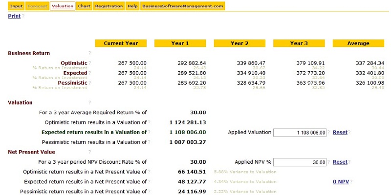
The Valuation Module applies the Forecast Analysis to generate a Business Valuation. The valuation is determined by the average Business Return (profit) over the forecast period and Required Return on Investment. Sensitivity Analysis provides Optimistic, Expected and Pessimistic business valuations. The Expected Valuation reflects the valuation for the most likely (Expected) return. Purchasing the business for an amount equal to the Expected Valuation provides an average Return on Investment equal to the Required Return %.
Calculation formula are provided for reference and to enable an in-depth understanding of the underlying calculations applied. Valuation can be completed without reference to the formula.
These are Module specific Controls. They appear as click-able links below the Analysis Menu.
This Control prints the current window. You can also use the browsers Print and Print Preview functions to set print variables. To do this from your browser tool bar go File, Print or File, Print Preview.
Business Return as calculated in the Forecast is provided for each Sensitivity (Optimistic, Expected and Pessimistic), for the Current Year, each Forecast Year and the Average of the Forecast Years. It is a true indicator of the return an investment in the business will provide.
Business Return reflects the before tax annual long term return of the business. It considers asset re-investment and any Owners external income forsaken.
It is is calculated as the Profit/Surplus less the Depreciation Allowance and less Owners External Earning Power.
Business Return = Profit/Surplus - Depreciation - Owners Earning Power
Optimistic Business Return is the Business Return where Relative Indicator values are adjusted by the Sensitivity % to improve the Forecast. It can be considered the best case scenario.
The % Return on Investment is based on the Applied Valuation, by default this is the Expected Valuation. This is the percentage the return the business provides for an investment (purchase price) equal to the Applied Valuation.
Expected Business Return is the Business Return where Relative Indicator values not adjusted by the Sensitivity %. It can be considered the most likely or average scenario.
The % Return on Investment is based on the Applied Valuation, by default this is the Expected Valuation. This is the percentage the return the business provides for an investment (purchase price) equal to the Applied Valuation.
Pessimistic Business Return is the Business Return where Relative Indicator values are adjusted by the Sensitivity % to degrade the Forecast. It can be considered the worst case scenario.
The % Return on Investment is based on the Applied Valuation, by default this is the Expected Valuation. This is the percentage the return the business provides for an investment (purchase price) equal to the Applied Valuation.
The Valuation is based on the Business Return and the Required Return % to determine a business valuation.
Optimistic Valuation is the value of the business based on the Average Optimistic Return divided by the Required Return %. It is the value of the business that provides the Required Return % when the Optimistic Business Return is achieved.
Optimistic Valuation = Average Optimistic Return / (Required Return % / 100)
The Average Optimistic Return is the average of Forecast Years only, it does not include the Current Year.
Expected Valuation is the value of the business based on the Average Expected Return divided by the Required Return %. It is the value of the business that provides the Required Return % when the Expected Business Return is achieved.
Expected Valuation = Average Expected Return / (Required Return % / 100)
The Average Expected Return is the average of Forecast Years only, it does not include the Current Year.
Pessimistic Valuation is the value of the business based on the Average Pessimistic Return divided by the Required Return %. It is the value of the business that provides the Required Return % when the Pessimistic Business Return is achieved.
Pessimistic Valuation = Average Pessimistic Return / (Required Return % / 100)
The Average Pessimistic Return is the average of Forecast Years only, it does not include the Current Year.
Applied Valuation is the valuation currently used in the % Return on Investment calculations for the Business Return and the Variance to Valuation calculations for the Net Present Value.
The Applied Valuation can be changed to review the impact on the Return on Investment. This effectively provides a reverse valuation where the Return on Investment can be determined for a set asking price.
The default Applied Valuation value is the Expected Valuation.
This is a click-able Control. When clicked Reset for the Applied Valuation returns the Applied Valuation value to the default value which is the Expected Valuation.
Net Present Value analysis is not required for Business Valuation. It is provided as an additional supporting methodology.
Net Present Value is the sum of current and future cash flows, where future cash flows are discounted to equivalent present values. It allows financial calculations relating to future events to be considered in present value terms allowing the cost of money, inflation, or opportunity cost to be factored into a financial calculation. This is done by discounting future cash flows to reflect that a dollar received today maybe worth more than a dollar received in a years time.
The longer the future time frame being considered the greater the importance of Net Present Value. For a time frame of 3 years it may provide little additional benefit, as the time frame increases it may become increasingly relevant.
However applying Net Present Value increases the complexity of calculations and tends to make them less intuitive. Therefore base valuations are calculated using the average forecast returns without discounting future cash flows.
From a valuation perspective Net Present Value is the sum of cash flows over the forecast period. This includes the price paid for the business as a negative cash flow (ie the Applied Valuation) and the future cash flows generated by the business (ie the Business Return for each Forecast Year) discounted to equivalent present values, and the potential value of the business at the end of the period.
If the Net Present Value is greater than 0 the investment return exceeds the discount rate (Applied NPV %) and it is a cash positive investment.
If the Net Present Value is equal to 0 the investment return matches the discount rate (Applied NPV %) and it is a cash neutral investment.
If the Net Present Value is less than 0 the investment return exceeds the discount rate (Applied NPV %) and it is a cash negative investment.
For additional detail see Net Present Value at Wikipedia.
Optimistic Net Present Value is the sum of the Applied Valuation (outgoing), the Net Present Value of the Optimistic Business Returns for each forecast year discounted by the Applied NPV %, and the future sale price discounted by the Applied NPV %. The % Variance to Valuation is the Optimistic Net Present Value expressed as a percentage of the Applied Valuation.
Optimistic Net Present Value =
- Applied Valuation
+ Sum of each Forecast Year [Optimistic Business Return / (1 + Applied NPV %) ^ Year]
+ Future Sale Price / (1 + Applied NPV %) ^ Year
The Future Sale Price is based on the the Optimistic Business Return of the Last Forecast Year and the Required Return %. Mouse over the calculated Net Present Value to display the Future Sale Price and the Future Sale Price Present Value (future sale price discounted by the Applied NPV %).
Future Sale Price = Optimistic Business Return of the Last Forecast Year / (Required Return %/100)
Expected Net Present Value is the sum of the Applied Valuation (outgoing), the Net Present Value of the Expected Business Returns for each forecast year discounted by the Applied NPV %, and the future sale price discounted by the Applied NPV %. The % Variance to Valuation is the Expected Net Present Value expressed as a percentage of the Applied Valuation.
Expected Net Present Value =
- Applied Valuation
+ Sum of each Forecast Year [Expected Business Return / (1 + Applied NPV %) ^ Year]
+ Future Sale Price / (1 + Applied NPV %) ^ Year
The Future Sale Price is based on the the Expected Business Return of the Last Forecast Year and the Required Return %. Mouse over the calculated Net Present Value to display the Future Sale Price and the Future Sale Price Present Value (future sale price discounted by the Applied NPV %).
Future Sale Price = Expected Business Return of the Last Forecast Year / (Required Return %/100)
Pessimistic Net Present Value is the sum of the Applied Valuation (outgoing), the Net Present Value of the Pessimistic Business Returns for each forecast year discounted by the Applied NPV %, and the future sale price discounted by the Applied NPV %. The % Variance to Valuation is the Pessimistic Net Present Value expressed as a percentage of the Applied Valuation.
Pessimistic Net Present Value =
- Applied Valuation
+ Sum of each Forecast Year [Pessimistic Business Return / (1 + Applied NPV %) ^ Year]
+ Future Sale Price / (1 + Applied NPV %) ^ Year
The Future Sale Price is based on the the Pessimistic Business Return of the Last Forecast Year and the Required Return %. Mouse over the calculated Net Present Value to display the Future Sale Price and the Future Sale Price Present Value (future sale price discounted by the Applied NPV %).
Future Sale Price = Pessimistic Business Return of the Last Forecast Year / (Required Return %/100)
Applied NPV % is the NPV Discount Rate % currently used in the Net Present Value calculations. It has no relationship to the Valuation calculations.
The Applied NPV % can be changed to review the impact on the Net Present Value calculations. This allows the Discount Rate to be adjusted to reflect a range of alternatives such as inflation, the cost of money, opportunity cost, or risk coverage.
The default Applied NPV % value is the Required Return %.
The value of the Required Return % would normally reflect the opportunity cost or risk coverage for an investment.
This is a click-able Control. When clicked Reset for the Applied NPV % returns the Applied NPV % value to the default value which is the Required Return %.
This is a click-able Control. When clicked 0 NPV % adjusts the Applied Valuation to a value resulting in an Expected Net Present Value of 0.
Breakeven Analysis applies your current performance input to determine breakeven points for Annual Revenue and Number of Sales. It applies the Annual Revenue, Total Variable, and Total Fixed values with the Breakeven Data values to calculate breakeven points.
To perform Breakeven Analysis values must be provided for Annual Revenue, Total Variable, and Total Fixed in the Input module. If you have undertaken a Forecast Analysis these vales will already be set. If you prefer to undertake a quick Breakeven Analysis without a forecast you can simply input an Annual Revenue value and set the Total Variable and Total Fixed values via the Other Variable and Other Fixed inputs with all other expenses set as 0.
Calculation formula are provided for reference and to enable an in-depth understanding of the underlying calculations applied. Breakeven analysis can be completed without reference to the formula.
These are Module specific Controls. They appear as click-able links below the Analysis Menu.
This Control prints the current window. You can also use the browsers Print and Print Preview functions to set print variables. To do this from your browser tool bar go File, Print or File, Print Preview.
This Control plots the Breakeven Analysis on the Chart module. It shows Annual Revenue and Total Expenses by Number of Sales. The Breakeven point is where Revenue and Expenses cross. Below this point the business surplus is negative (loss) and above this point the business surplus is positive (profit). The amount of surplus is the difference between the Annual Revenue and Total Expenses.
This is the current Annual Revenue input value from the Input module.
This is the current Average Sale Price input value from the Input module.
This is the current Number of Sales calculated value from the Input module.
Number of Sales = Annual Revenue / Average Sale Price
This is the current Total Variable expenses calculated value from the Input module. It is the sum of the variable expenses.
This is the current Total Fixed expenses calculated value from the Input module. It is the sum of the fixed expenses.
This is the current Profit/Surplus calculated value from the Input module. It is the revenue less total expenses.
Profit/Surplus = Annual Revenue - (Total Variable + Total Fixed)
This is the current revenue required for the business to breakeven.
Breakeven Revenue = Total Fixed / ( 1 - (( Total Variable / Number of Sales ) / Average Sale Price ))
this is equivalent to
Breakeven Revenue = Total Fixed / ( 1 - ( Variable Expense per Sale / Average Sale Price ))
Revenue less than breakeven revenue results in a loss. Revenue greater than breakeven revenue results in a profit.
This is the current number of sales required for the business to breakeven.
Breakeven Number of Sales = Breakeven Revenue / Average Sale Price
Less than the breakeven number of sales results in a loss. Greater than breakeven number of sales results in a profit.
Price Analysis applies current Annual Revenue, Total Variable, and Total Fixed values with the Price Data values to project business surplus over a range of prices. It allows you to test the impact of pricing changes on revenue and surplus. Price Analysis projects outcomes for pricing from 50% to 200% of the current price and calculates the optimum price. The optimum price provides the highest surplus (profit).
Price Analysis requires Breakeven Analysis be completed.
Calculation formula are provided for reference and to enable an in-depth understanding of the underlying calculations applied. Price analysis can be completed without reference to the formula.
These are Module specific Controls. They appear as click-able links below the Analysis Menu.
This Control prints the current window. You can also use the browsers Print and Print Preview functions to set print variables. To do this from your browser tool bar go File, Print or File, Print Preview.
This Control plots the Price Analysis on the Chart module. It shows Annual Revenue and Profit/Surplus by Average Sale Price. The optimum Average Sale Price is where Profit/Surplus is highest.
By stepping through price ranges of 50% to 200% of the current Average Sale Price, calculating the corresponding Profit/Surplus and identifying the point of maximum Profit/Surplus the optimum Average Sale Price is determined.
This is the price that provides the highest surplus (profit) for the business.
It is determined by using Step Values of 0.5 to 2.0 (ie 50% to 200%) of the current Average Sale Price to step through price ranges, calculating the corresponding Profit/Surplus based on the Price change data and identifying the price providing the maximum Profit/Surplus.
The calculations for Profit/Surplus at each price point apply the Sales Price Ratio.
Sales Price Ratio = Sale Price Change % / Number of Sales Change %
Using Example Business Data
Sales Price Ratio = -15 / 20 = -0.75
This is the number of sales at the Optimum Average Sale Price.
Optimum Number of Sales = ( 1 + (Step Value - 1) * Sales Price Ratio ) * Number of Sales
Using Example Business Data with an Optimum Average Sale Price of 140 which is a Step Value of 1.4 (ie a 140% change on the Average Sale Price of 100).
Optimum Number of Sales = ( 1 + ((1.4 - 1) * -0.75)) * 10 000 = 0.7 * 10 000 = 7000
This is the annual revenue at the Optimum Average Sale Price.
Optimum Annual Revenue = Optimum Number of Sales * Optimum Average Sale Price
Using Example Business Data:
Optimum Annual Revenue = 7000 * 140 = 980 000
This is the total variable expenses at the Optimum Average Sale Price.
Optimum Total Variable = Optimum Number of Sales * ( current Total Variable / current Number of Sales )
Using Example Business Data:
Optimum Total Variable = 7000 * ( 450 000 / 10 000 ) = 315 000
This is the total fixed expenses at the Optimum Average Sale Price.
Optimum Total Fixed = current Total Fixed
Using Example Business Data:
Optimum Total Fixed = 170 000
This is the total surplus at the Optimum Average Sale Price.
Optimum Profit/Surplus = Optimum Annual Revenue - ( Optimum Total Variable + Optimum Total Fixed )
Using Example Business Data:
Optimum Total Fixed = 980 000 - ( 315 000 + 170 000 ) = 495 000
The Chart Module provides a plot of selected data by Year. It includes the Current Year (Year 0) and each Forecast Year. Plot data for Breakeven and Price analysis is also added to the Chart from the Breakeven and Price Modules.
Forecast and Valuation Modules
Plot data is added to the Chart from the Forecast or Valuation Modules by clicking the label of the required data set. This can be repeated to add multiple data sets. The chart is designed to display up to 3 data sets at once each in a different color. The data set plot color is determine by the order it is added to the chart. The first plot is Green, second Red, and third Blue. Plotting Expected, Optimistic and Pessimistic values in order from the Valuation Module results in Optimistic (green), Pessimistic (red), Expected (blue). When more than 3 data sets are added colors are repeated. As data sets are added there is a negative impact on performance. A maximum of 3 data sets is recommended.
Both values and percentages can be plotted. Click to Plot is displayed when the mouse moves over a plot table data set label in the Forecast or Valuation Modules. All plotted data sets use the same Y-axis.
In the Chart the Label of the plotted data is displayed as a title at the top of the Chart in the same color as the plot. Click to Clear is displayed when the mouse moves over a title Label. When a title Label is clicked the plot for that data will be Cleared from the chart. Each plot includes square markers at each Year point. The data value at that point is displayed when the mouse moves over a square marker.
Breakeven and Price Modules
Plot data is added to the Chart from the Breakeven and Price Modules by clicking the top Plot Control for the module.
The Plot Breakeven control plots the Breakeven Analysis on the Chart module. It shows Annual Revenue and Total Expenses by Number of Sales. The Breakeven point is where Revenue and Expenses cross. Below this point the business surplus is negative (loss) and above this point the business surplus is positive (profit). The amount of surplus is the difference between the Annual Revenue and Total Expenses.
The Plot Price control plots the Price Analysis on the Chart module. It shows Annual Revenue and Profit/Surplus by Average Sale Price. The optimum Average Sale Price is where Profit/Surplus is highest.
These are Module specific Controls. They appear as click-able links below the Analysis Menu.
This Control Clears the Chart removing all plots and axis.
This Control prints the current window. You can also use the browsers Print and Print Preview functions to set print variables. To do this from your browser tool bar go File, Print or File, Print Preview.
Business Analysis Access/Download Help License +bizpep.com
License Business Analysis
Please consider supporting application development. Licensing your application will fully enable all functions.
Secure online transaction processing is provided via PayPal. License details are sent by email as soon as your transaction is processed and will fully enable your application.
Business Analysis
$99.00 USD License Fee
Your one time perpetual license fully enables application use on multiple devices for the individual licensed email address recipient.
Registration details are processed and confirmation sent by email as soon as your transaction is processed. When your confirmation email is received simply select Registration from the application menu and submit your Registration Details.
Application suitability must be independently assessed and use indicates acceptance of any and all associated risk.
Thank you for supporting continued application development.
Business Analysis Access/Download Help License +bizpep.com
